In the evolving landscape of 3D digitization,
the widespread adoption of advanced scanning technologies is frequently impeded by two primary factors:
the prohibitive cost associated with the integration of an excessive
number of components in commercial systems, and a pervasive lack of transparency regarding their control mechanisms.
While open-source initiatives, such as the HSKAnner from Karlsruhe,
demonstrate the potential for community-driven development,
they often rely on fixed multi-camera arrays, which, despite their open nature, can still contribute to elevated costs and architectural rigidity.
HSKAnner 3D Scanner from Karlsruhe
This project introduces I-Scan, a novel 3D scanner designed to address these limitations
by prioritizing universality, cost-efficiency, and unparalleled modularity.
I-Scan is engineered for broad sensor compatibility,
supporting a diverse range of imaging devices, including legacy USB and web cameras (which are currently implemented),
and is extensible to integrate various other measurement units such as Lidar or general Time-of-Flight (ToF) sensors,
or indeed any sensor where precise spatial positioning is advantageous.
A core design principle is its adaptable architecture,
where modules possess spatial awareness and are reconfigurable to suit specific use-case requirements,
thereby obviating the need for a singular, fixed setup.
The integration of movable modules along the Z-axis,
coupled with servo-controlled adjustable camera angles,
facilitates comprehensive image acquisition across varying object heights and perspectives,
enhancing data capture flexibility.
The operational backbone of I-Scan is a robust Python based application.
This software orchestrates critical functions, including the import and configuration of cameras via JSON files (supporting COM and HTTP interfaces),
precise calculations for Z-axis module movement,
and servo alignment for camera orientation, all managed through REST APIs.
Furthermore, the application provides capabilities for defining complex scan workflows,
visualization of scanner settings, rigorous input validation (mathematical and JSON syntax),
automated dependency management, and comprehensive debug output.
This holistic approach positions I-Scan as a highly adaptable, cost-effective, and transparent solution,
poised to democratize access to advanced 3D digitization capabilities.
The conceptual foundation of this 3D scanner is a modular, highly adaptable structure
that integrates movable and stationary modules for precise, customizable, and efficient object digitization.
Central is the dynamic interaction between modules, each with spatial awareness and distinct degrees of freedom,
enabling the system to overcome the limitations of conventional fixed array scanners.
Movable modules traverse the Z-axis with high positional accuracy,
guided by user defined or algorithmically determined center points in 3D space.
At each increment, these modules reorient their sensors (e.g., cameras)
so their optical axes converge on the current target center.
This is achieved through coordinated actuation of stepper motors (linear displacement)
and servo motors (angular adjustment), all managed via a REST API.
The mathematical logic ensures that, regardless of Z-axis position,
the sensor maintains optimal focus and perspective.
Fixed modules are strategically positioned and, while stationary,
can dynamically target new center points, mirroring the adaptive behavior of movable modules.
This combination enables flexible and efficient scan paths,
accommodating a wide variety of object geometries and sizes.
This modularity enhances coverage and resolution
and allows individualized scan trajectories tailored to the object's morphology.
All control operations from positioning to sensor orientation are abstracted through a unified REST API,
ensuring integration, extensibility, and remote operability.
The mathematical framework enables each module to compute the necessary transformations
for precise alignment with dynamically assigned center points.
This approach makes the scanner a versatile platform for advanced 3D digitization
in research and industrial applications.
By vertically displacing along the Z-axis and dynamically adjusting sensor angles, the movable modules generate significantly more perspectives than rigid fixed array setups (where all sensors are locked in pre-defined positions and orientations, offering no adaptability during operation).
This eliminates "blind spots" and enables gapless digitization of complex geometries, overcoming the physical constraints of static camera positions.
Such systems fundamentally limit perspective coverage to their initial hardware configuration, causing unavoidable blind spots on non convex surfaces.
(Non-convex surfaces exhibit cavities, undercuts, or reentrant angles where direct "line of sight" is obstructed – e.g., gear teeth, hollow sculptures, or organic structures like tree roots).
Through its modular architecture, the system achieves exceptional flexibility,
enabling seamless integration and adaptation of diverse sensors without requiring full hardware reconfiguration.
Future implementations will leverage sensor fusion pipelines to optimize 3D data acquisition and processing
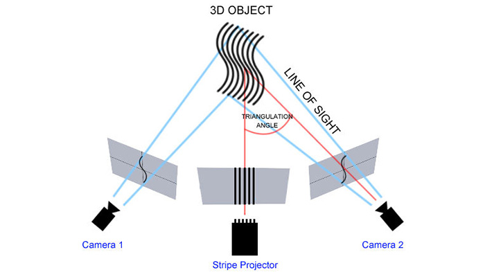
for instance, by combining cameras with LiDAR or ToF sensors. This extensibility inherently supports advanced techniques like structured light scanning, where projected patterns and multi angle triangulation reconstruct complex surface geometries with sub millimeter accuracy.
In this chapter, we show how to calculate the angle α in a right-angled triangle when one side is variable.
For our example:
Side A:Zdist
Side B:DistanceToCenter (150 cm as defined in the JSON configuration)
In a right-angled triangle, the tangent of an angle is defined as the ratio of the opposite side to the adjacent side.
Since α is the angle opposite Side A and Side B is the adjacent side, it follows:
tan(α) = Zdist / DistanceToCenter
To calculate α, use the arctangent (inverse tangent) function:
α = arctan(Zdist / DistanceToCenter)
Example:
With Zdist = 150 cm and DistanceToCenter = 150 cm:
α = arctan(150 / 150) = arctan(1) = 45°
This method allows you to substitute any value for Zdist to calculate the corresponding angle α in a right-angled triangle.
To ensure that each servo can be installed regardless of its individual angular range,
the servo parameters are configured accordingly.
By specifying the installation angle of the servo, we can align it precisely.
The servo’s cone of rotation is combined with the installation angle
and then matched with the theoretically calculated angle to the object.
This process yields the exact angle at which the servo must be controlled
to achieve the desired orientation as previously determined by the geometric calculations.
For each measurement point, the algorithm calculates the geometric angle,
determines the target angle in the coordinate system,
checks if the target is within the servo’s physical range,
and maps this to the actual servo angle.
All relevant values are stored for further control and visualization.
For a single measurement point:
Calculate target angle, check reachability, map to servo angle, calculate visualization angle, and store all values in the result object.
The user interface provides a powerful way to create and manage scan workflows.
Each step of the 3D acquisition process can be defined in detail.
A workflow consists of multiple steps that are executed sequentially to ensure a structured and repeatable scanning procedure.
Each step in the workflow is individually configurable.
This includes not only Z-axis movement, servo alignment, and camera control,
but also the integration of multiple cameras into the process.
Cameras can be added to the workflow as needed,
and each camera can be fully configured through the interface.
Camera parameters can be adjusted, active cameras for specific steps can be selected,
and their operation can be coordinated with other system components.
Future features such as lighting control can also be integrated into the workflow,
providing even more flexibility and control.
This approach allows all relevant settings for each step to be reviewed, adjusted, and optimized.
In this window, as described in the previous chapter, you can set the variables for the scan.
The visualization mode generates a full visual evaluation of all results, while silent mode creates a CSV file based on the parameters.
The CSV file is automatically imported into the queue window.
The current command field helps you understand how to use the math engine if you want to integrate it elsewhere.
You can also select Cone details to view the configuration in detail.
The Camera JSON Configurator is located at the bottom right of the software interface.
It allows you to conveniently adjust camera settings via a JSON file.
Parameters such as resolution, frame rate, and exposure can be modified directly in the configurator.
Changes are immediately reflected in the camera's live view.
Cameras can currently be imported into the software either via a COM port (e.g., USB camera) or via a stream (e.g., IP camera).
The configuration stores important camera information, which can later also be used in external software such as Meshroom.
To ensure reliability, the JSON file is automatically checked for correct syntax with every change.
If there are errors with the camera connection, an error message will be displayed in the console window.
Additionally, the UI will show an error message describing the issue.
With this system, each camera’s spatial vector is precisely known and documented. You can define a fixed scanning area and extract all possible perspectives that the setup allows. All relevant camera positions, scan area, and workflow steps are easily accessible from JSON or CSV files, including camera configuration and scan settings.
This accelerates processing in Meshroom, as the determination of camera positions can be almost skipped. Consistency is ensured: if you later add more images taken from the same known positions, they can be seamlessly integrated into the existing reconstruction without recalculating the entire structure from scratch.
Direct transfer of known camera positions to Meshroom is planned as the next feature, but it is not yet implemented.
Until then, Meshroom will continue to determine camera positions.
Meshroom is an open-source software for photogrammetric 3D reconstruction,
developed by AliceVision.
It enables the automatic creation of detailed 3D models from a series of photos of an object or scene.
Meshroom provides a graphical user interface
where the entire workflow, from image selection and feature detection,
camera calibration, dense point cloud calculation, to mesh and texture generation
is visually represented as a pipeline.
The software uses advanced image processing algorithms
and is completely free to use.
Meshroom also includes algorithms that can infer camera positions
by analyzing the overlap between images.
The image shows the default pipeline in Meshroom. Each node represents a processing step in the photogrammetry workflow, from image input to 3D model output.
This example shows a coordinated scan of a metallic object placed on a white surface, with illumination coming from one side (as indicated by the visible shadow). Despite the typical complications associated with scanning reflective or metallic materials, the system successfully detected and reconstructed all non-metallic features of the object.
This section presents the UML diagrams and API documentation for the I-Scan software. The class diagram provides an overview of the main modules and their relationships, and allows you to explore available functions along with their descriptions. Use the collapsible tables below to view detailed information about each function and its purpose within the system.
Note: If diagrams or similar visual elements do not load, simply reload the page.
Currently, no optimized images are available on the site.
 GitHub Repository Software Version 1.0:
Release V1.0 I-Scan
GitHub Repository Software Version 1.0:
Release V1.0 I-Scan